2 Avian blood parasites

# Load required packages
# Data manipulation
library(tidyverse)
library(DT)
library(here)
# Modeling
library(mrIML)
library(tidymodels)
library(future)
library(finetune)
library(flashlight)
# Plotting
library(igraph)
library(ggnetwork)
library(cowplot)
library(patchwork)

# Load custom functions
source(here("R-functions", "select_variables.r"))
source(here("R-functions", "plot_network.r"))

# Set up parallel processing
n_cores <- parallel::detectCores()
plan("multicore", workers = 2)

# Set seed
set.seed(1234)

This case study demonstrates the application of MrIML 2.0 to a small dataset of vector-borne blood parasites in New Caledonian birds. We analyze presence/absence data from four parasite species:

Haemoproteus zosteropis species complex
H. killangoi species complex
Plasmodium spp.
Nematode Microfilaria species

The dataset includes 449 individual birds and a covariate representing the proportion of captures attributed to Zosterops spp. at each site, serving as a proxy for host relative abundance.

data <- MRFcov::Bird.parasites
datatable(data)

To prepare the data for multi-response modeling, we separate it into Y (response), X (predictors), and X1(co-occurrence predictors). This is how data is parsed to mrIML.

# Prepare response variables (parasite species)
Y <- data %>%
  dplyr::select(-scale.prop.zos) %>%
  dplyr::select(sort(names(.)))

# Prepare predictor variables (host abundance proxy)
X <- data %>%
  dplyr::select(scale.prop.zos)

# Co-occurrence data (other parasites as predictors)
X1 <- Y %>%
  dplyr::select(sort(names(.)))

2.1 Model definition

We formulate three models of community assembly to compare the relative importance of co-occurrence versus environmental effects:

Parasite co-occurrence only (just X₁, no other covariates)
Host abundance only (just X, the ‘host abundance model’)
Combined model (both X₁ and X, co-occurrence + host abundance)

However, all three of these model configerations utilise the same base random forest model specified using tidymodels.

# Define random forest model
model_rf <- rand_forest(
  trees = 1000,
  mode = "classification",
  mtry = tune(),
  min_n = tune()
) %>%
  set_engine("randomForest")

2.1.1 Model 1: Combined model (co-occurrence + host abundance)

yhats_rf_combined <- mrIMLpredicts(
  X = X,
  Y = Y,
  X1 = X1,
  Model = model_rf,
  balance_data = 'no',
  tune_grid_size = 5,
  prop = 0.7,
  k = 5,
  racing = TRUE
)

i Creating pre-processing data to finalize 1 unknown parameter: "mtry"
i Creating pre-processing data to finalize 1 unknown parameter: "mtry"
i Creating pre-processing data to finalize 1 unknown parameter: "mtry"
i Creating pre-processing data to finalize 1 unknown parameter: "mtry"

2.1.2 Model 2: Host abundance only

yhats_rf_nox1 <- mrIMLpredicts(
  X = X,
  Y = Y,
  X1 = NULL,
  Model = model_rf,
  balance_data = 'down',
  tune_grid_size = 5,
  prop = 0.7,
  k = 5,
  racing = TRUE
)

i Creating pre-processing data to finalize 1 unknown parameter: "mtry"
i Creating pre-processing data to finalize 1 unknown parameter: "mtry"
i Creating pre-processing data to finalize 1 unknown parameter: "mtry"
i Creating pre-processing data to finalize 1 unknown parameter: "mtry"

2.1.3 Model 3: Co-occurrence only

yhats_rf_nox <- mrIMLpredicts(
  X = NULL,
  Y = Y,
  X1 = X1,
  Model = model_rf,
  balance_data = 'down',
  tune_grid_size = 5,
  prop = 0.7,
  k = 5,
  racing = TRUE
)

i Creating pre-processing data to finalize 1 unknown parameter: "mtry"
i Creating pre-processing data to finalize 1 unknown parameter: "mtry"
i Creating pre-processing data to finalize 1 unknown parameter: "mtry"
i Creating pre-processing data to finalize 1 unknown parameter: "mtry"

2.2 Model performance

The proformance of each model for the diferen taxa can be explored using mrIMLperformance(). Below is an example for the combined model.

ModelPerf_combined <- mrIMLperformance(yhats_rf_combined)

Warning: NAs produced when calculating MCC. This is common when there is a
class imbalance. Substituting NA values with zero.

ModelPerf_combined$model_performance

# A tibble: 4 × 8
  response     model_name roc_AUC   mcc sensitivity   ppv specificity prevalence
  <chr>        <chr>        <dbl> <dbl>       <dbl> <dbl>       <dbl>      <dbl>
1 Hkillangoi   rand_fore…   0.851 0.366       0.983 0.908       0.25      0.116 
2 Hzosteropis  rand_fore…   0.901 0.649       0.93  0.894       0.694     0.265 
3 Microfilaria rand_fore…   0.954 0           1     0.926       0         0.0980
4 Plas         rand_fore…   0.907 0.369       0.936 0.857       0.370     0.196

We compare the three model configerations against one another based on average AUC.

# Evaluate model performance
ModelPerf_noX1 <- mrIMLperformance(yhats_rf_nox1)
ModelPerf_noX <- mrIMLperformance(yhats_rf_nox)

tibble(
  Model = c(
    "Combined model",
    "Host abundance only",
    "Co-occurrence only"
  ),
  AUC = c(
    ModelPerf_combined$model_performance$roc_AUC %>%
      mean(),
    ModelPerf_noX1$model_performance$roc_AUC %>%
      mean(),
    ModelPerf_noX$model_performance$roc_AUC %>%
      mean()
  ) %>%
    round(., 3)
)

# A tibble: 3 × 2
  Model                 AUC
  <chr>               <dbl>
1 Combined model      0.903
2 Host abundance only 0.814
3 Co-occurrence only  0.674

The combined model shows improved performance over the individual components, suggesting that both co-occurrence patterns and host abundance contribute to parasite distribution patterns, however this is a small dataset and so there is significant variation in the metric depending on the cross-validation and test-training split.

2.3 Bootstrap Analysis for Uncertainty Estimation

From here on, we focus on the combined model. However, we can use bootstraping to capture the uncertainty.

# Run bootstrap analysis for uncertainty estimation
bs_avian <- yhats_rf_combined %>%
  mrBootstrap(num_bootstrap = 100)

# Calculate variable importance with bootstrap confidence intervals
bs_impVI <- mrVip(
  yhats_rf_combined,
  mrBootstrap_obj = bs_avian,
  threshold = 0.0,
  global_top_var = 10,
  local_top_var = 5,
  model_perf = ModelPerf_combined
)

# Display variable importance plot
bs_impVI[[3]]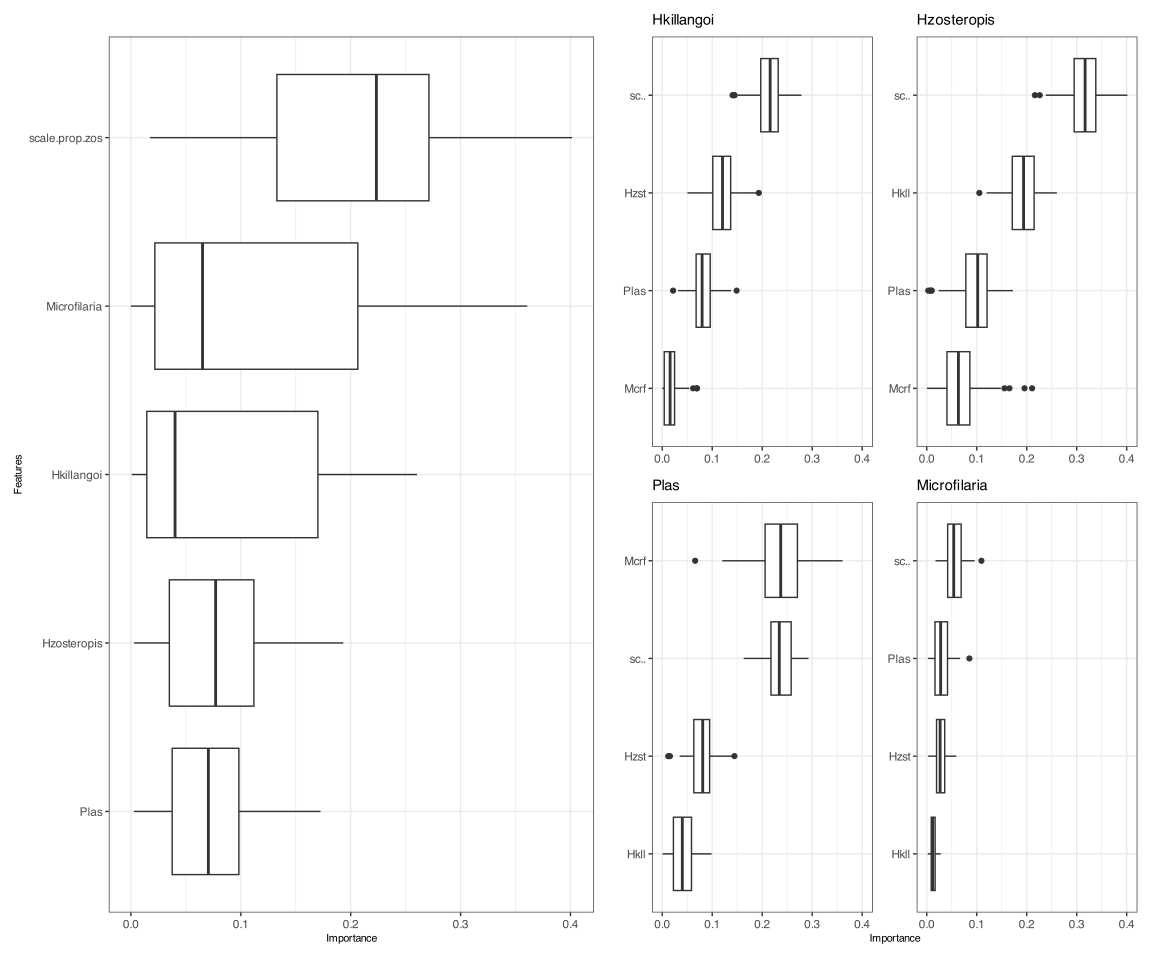

2.4 Partial Dependence Analysis

# Create bootstrapped partial dependence plots for Plasmodium
pds <- mrPdPlotBootstrap(
  yhats_rf_combined,
  mrBootstrap_obj = bs_avian,
  vi_obj = bs_impVI,
  target = 'Plas',
  global_top_var = 5
)

# Display partial dependence plots
pds[[2]]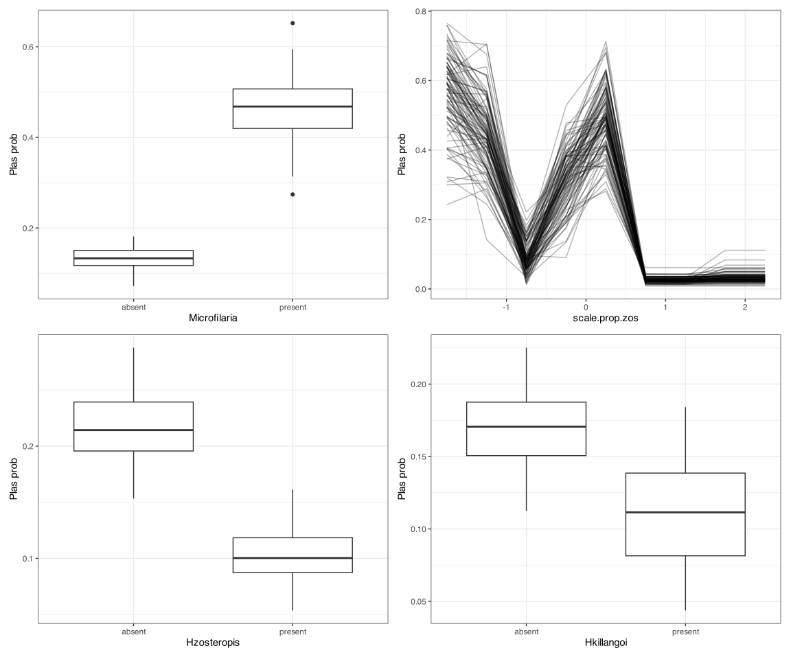

2.5 Environmental Covariate Effects

# Examine the relationship between host abundance and parasite occurrence
covar <- mrCovar(
  yhats_rf_combined,
  var = 'scale.prop.zos',
  sdthresh = 0.01
)

# Display the three components of covariate analysis
covar[[1]] / covar[[2]] / covar[[3]]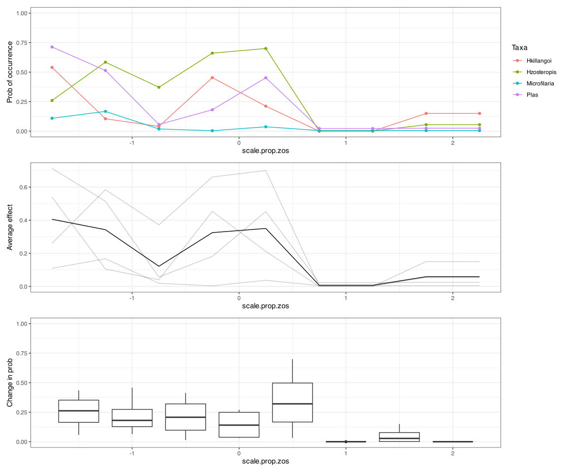

2.6 Interaction Analysis

# Analyze feature interactions using H-statistics
int_ <- mrInteractions(
  yhats_rf_combined,
  num_bootstrap = 100,
  feature = 'Plas',
  top_int = 10
)

# Display interaction plots
int_[[1]] / int_[[2]] / int_[[3]]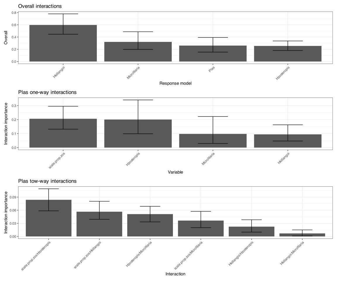

2.7 SHAP Analysis for Individual Predictions

# Perform SHAP analysis for detailed feature attribution
shap_results <- mrShapely(
  yhats_rf_combined,
  taxa = "Plas",
  plot_feature_effects = TRUE,
  plot_dependencies = TRUE,
  plot_2D_dependencies = TRUE
)

Exact Kernel SHAP values

p <- (shap_results$dependencies2D$Plas[[2]][[2]] +
  scale_colour_viridis_c(limits = c(-0.4, 0.8), option = "B") +
  theme_minimal() +
  labs(title = "b)")) +
  (shap_results$dependencies2D$Plas[[1]][[2]] +
    scale_colour_viridis_c(limits = c(-0.4, 0.8), option = "B") +
    theme_minimal() +
    labs(title = "c)")) +
  patchwork::plot_layout(ncol = 2, guides = "collect")

Scale for colour is already present.
Adding another scale for colour, which will replace the existing scale.
Scale for colour is already present.
Adding another scale for colour, which will replace the existing scale.

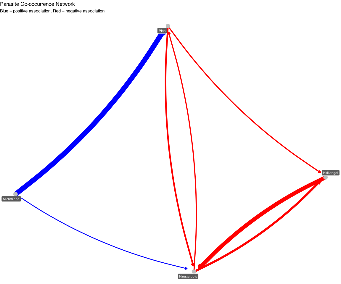
2.8 Co-occurrence Network Construction

# Build co-occurrence network from bootstrap results
assoc_net <- mrCoOccurNet(bs_avian)

plot_network(
  assoc_net,
  strength_threash = 0.05,
  network_title = "Parasite Co-occurrence Network"
)